
Forecasting Market Interest Rates Using Time Series & Neural Network Models In Data Science

Introduction
Market interest rates play a vital role in our economy. Interest rates will have a direct impact on money circulation and the economic activities in the country. By having an informed prediction of the movement of interest rates, markets can pre-emptively adapt to changing conditions. Forecasting of lending interest rate is a challenging task. Lending interest rates are influenced by many external and internal factors. This project intends to develop a predictive model that can forecast the Average Weighted Prime Lending Rate (AWPLR) based on historical data and relevant economic indicators.
Dependent variable selection
The AWPR is calculated by the Central Bank of Sri Lanka (CBSL) weekly, based on commercial bank's lending rates offered to their prime customers during a particular week. A monthly average of weekly AWPLR is also published. AWPLR has a direct impact on market interest rates since banks’ lending rates for corporates and individuals are mainly decided by the AWPLR.
Independent variables selection
AWPLR rates fluctuate due to many factors and have selected only the main factors, that can have a direct impact on AWPLR.
TbRate - Weekly 364 days Treasury bill rate
Inflation - Headline Inflation (Y-O-Y)
SDFR - Standing Deposit Facility Rate
SDFR provides the floor rate for absorbing overnight excess liquidity from the banking system by the Central Bank.
SLFR - Standing Lending Facility Rate
The interest rate applicable on reverse repurchase transactions of the Central Bank with Commercial banks on an overnight basis under the Standing Facility provides the ceiling rate for the injection of overnight liquidity to the banking system by the central bank.
AWFDR - Average Weighted Fixed Deposit Rate
A rate computed monthly based on all deposit rates of commercial banks, weighted by the outstanding deposit balances at the end of each month.
BankRate - Bank Rate
The rate at which the Central Bank grants advances to commercial banks for their temporary liquidity purposes.
USDLKRrate - Indicative Rate of the USD/LKR Exchange Rate
Prediction Models
Two major models have been used for forecasting of average weighted prime lending rate.
1. Time series models
2. Neural Network models
Data
Retrieved all the data for the project from the website of the Central Bank of Sri Lanka (www.cbsl.com), which is a platform holding statistical data for various interest rate-related data. Weekly figures (from 03.01.2020 to 26.05.2023) have been gathered to train the models. The dataset used was downloaded as Excel files, and then it was filtered and rearranged for training as well as testing purposes.
Model development
Both Time series models and Neural Network models have been used to analyze and interpret datasets. The intention of using two models for forecasting was to compare and see the accuracy level of each model for forecasting.
Time Series Analysis
Time series analysis is a technique in statistics that deals with time series data and trend analysis.
Implementation Process and Execution
Below are the imported libraries and packages needed for building the time series model.
Packages
tseries is a package developed by R CRAN. Use for time series data analysis. Can create time series
objects by using the ts() function by organizing the data such as frequency, starting year ending year, are this quarterly
data, monthly data, weekly data, etc. lubridate() package required for decimal dates. Since this is a weekly data there is a decimal number of weeks (365.25/7).
Fpp package required for forecasting.
Plotting of time series
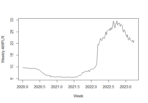
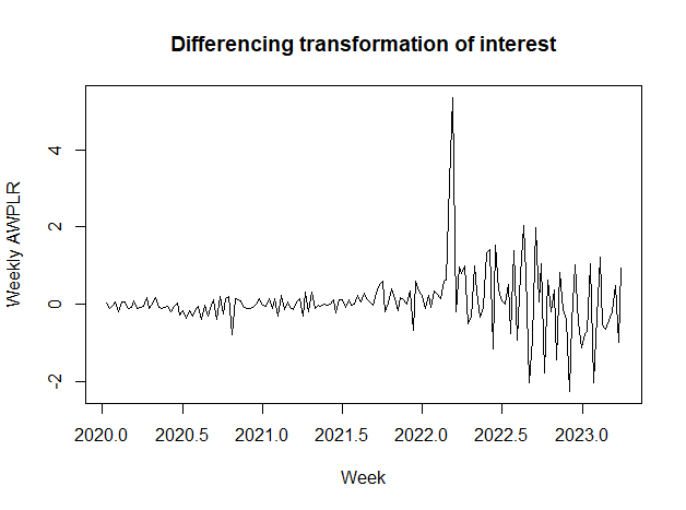
The series doesn’t show any clear trend component. There is an unusual hike between 2022.5 & 2023. We can consider that as an outlier. To get a clear idea about the series we need to plot ACF & PACF.
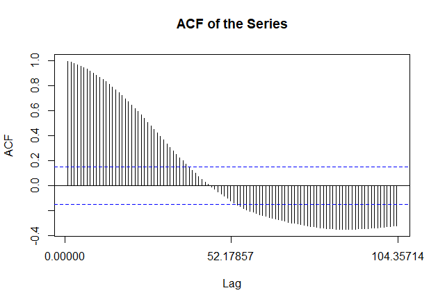
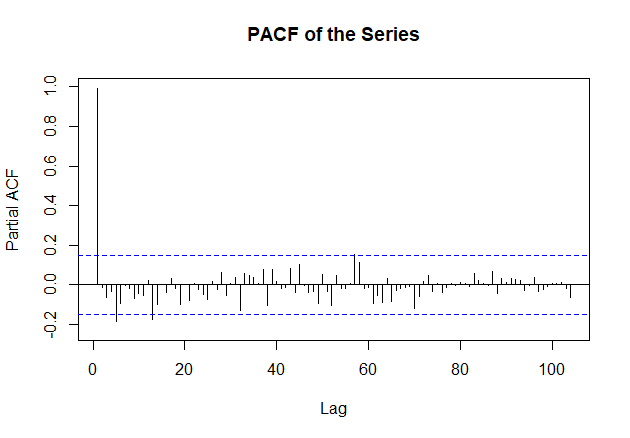
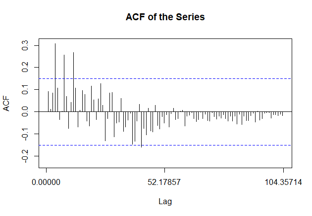
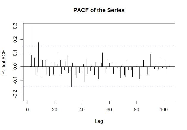
ACF function gives MA(q) & PACF function gives AR(p). According to ACF series seems to be nonstationary. Applied ADF to see whether it is stationary or not.
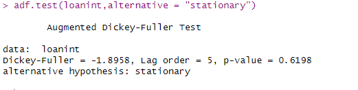
Since P value is > 0.05 we can’t reject the null hypothesis, which is series is not stationary. Since series is not stationary, we can apply a differencing transformation technique to make it stationary. ndiffs function can be used to identify the number of differences
Plotting of differencing transformation of interest
Adf test after differencing
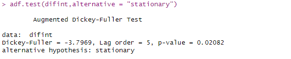
since p value <0.05, series is stationary. ACF & PACF plots after differencing.
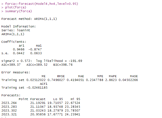
Use of AUTO ARIMA function to the original dataset (loanint) & the differencing dataset (difint) to identify the best forecasting model. A model with the lowest AIC can be considered the best fit.
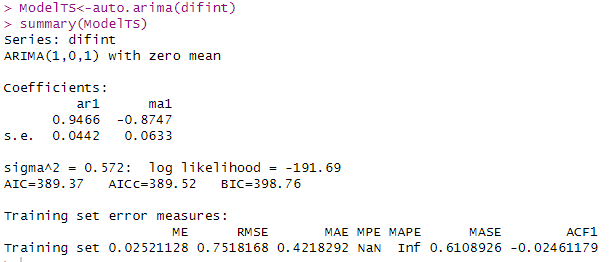
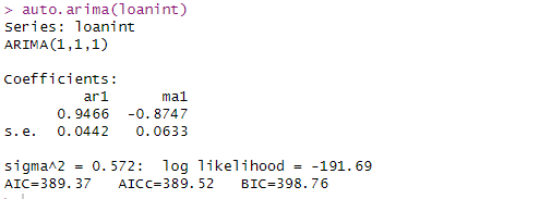
Since both the models are closely matched, the ARIMA for neighboring models to identify the best model.
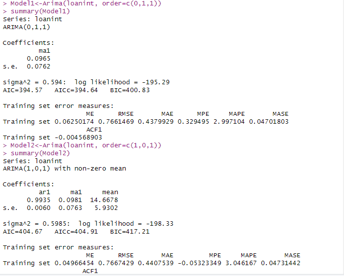
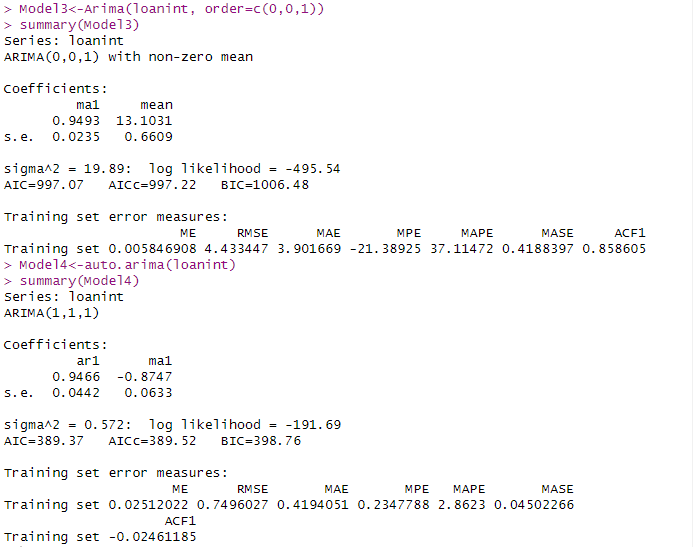
It shows that Model4 is the best fit.
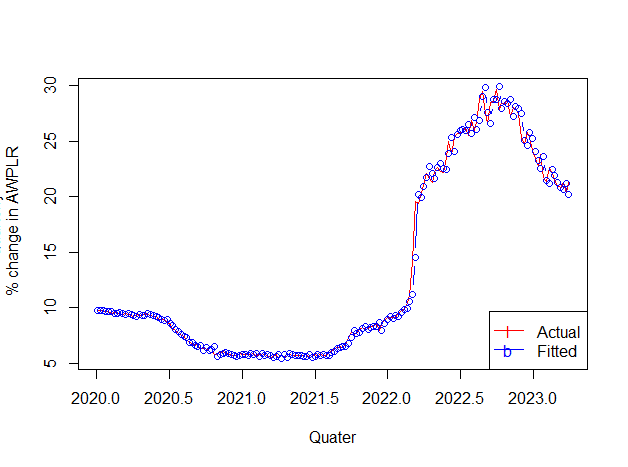
Comparing the fitted values with actuals.
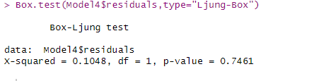
Box.test(Model4$residuals,type="Ljung-Box")
# H0: The residuals are independently distributed.
HA: The residuals are not independently distributed;
P-value of the test is 0.7461, which is much larger than 0.05. Thus, we fail to reject the null hypothesis of the test and conclude that the data values are independent.
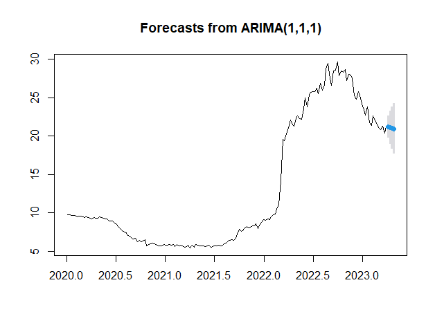
Forecasting for 4 weeks

Neural Network Model
Implementation Process and Execution
Below are the imported libraries and packages needed for building the time series model.
Structure of the dataset
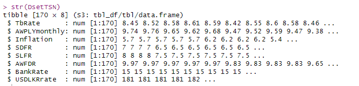
For the training and testing of our dataset, we decided to train 75% of the data and test the remaining 25%.

To normalize our data, we needed to do data scaling which is a pre-processing step recommended when working on deep learning algorithms. The data in the training set was scaled for simplification purposes.

We have to get a train & test set from the transformed data series.
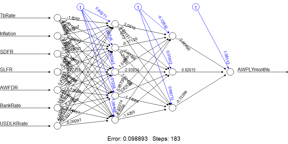
Fitting the ANN model to the training set
>nn <- neuralnet(f,data=train_,hidden=c(5,3),linear.output=T)
> plot(nn)
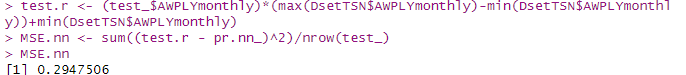
Calculating the mean squared error of the ANN in the test set.
Mean squared error consists of actual values minus predicted values & getting the summation of those values and dividing it by several observations. For that, we need predicted values and actual values as well
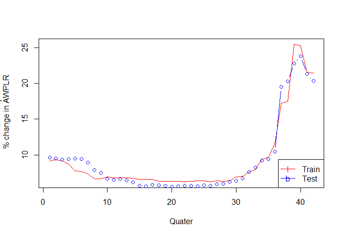
Comparing the fitted values of Train & Test sets.
Fitting a regression model for the same scenario
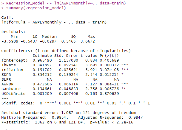
comparing the two errors in the test set
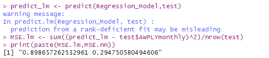
The neural network model has reported a lower MSE than the linear regression model.
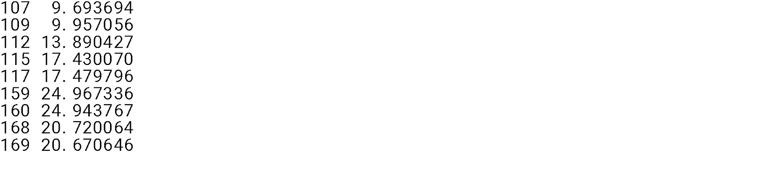
Given below are some of the selected forecasted values. 169 represents the AWPLR as of 26th May 2023 or rate as of the 169th week.
Conclusions
Out of the two models used it shows that Neural network models give more accurate predictions mainly because more independent variables have been used in contrast to the use of only one variable in time series analysis. The stability of the neural network results with different network parameters should be investigated further and should examine other factors, which influence the AWPLR other than the variables used.
References
CBSL (2019). Monetary Policy | Central Bank of Sri Lanka. [online] Cbsl.gov.lk. Available at: https://www.cbsl.gov.lk/en/monetary-policy/about-monetary-policy.


